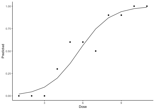
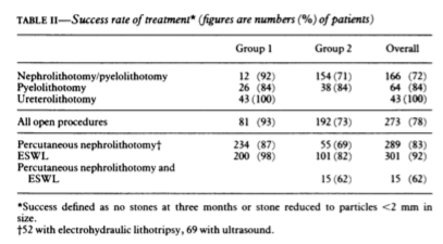
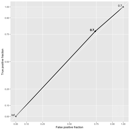
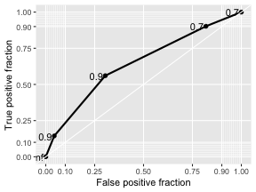
class: center, middle, inverse, title-slide # Logistic Regression ## STA2453 ### Nathan Taback ### 2019-10-08 --- ## Example This example is based on Efron and Hastie (2016). - An experimental new anti-cancer drug called Xilathon is under development. - Before human testing can begin, animal studies are needed to determine safe dosages. - A dose–response experiment was carried out: 11 groups of `\(n=10\)` mice each were injected with increasing amounts of Xilathon, dosages coded as `\(1, 2, \dots, 11\)`. --- .pull-left[ ```r library(tidyverse) library(broom) doseresponse <- read_table2("https://web.stanford.edu/~hastie/CASI_files/DATA/doseresponse.txt") doseresponse$Dose <- 1:11 ``` ```r doseresponse %>% head(7) ``` ``` ## # A tibble: 7 x 2 ## Dose Proportion ## <int> <dbl> ## 1 1 0 ## 2 2 0 ## 3 3 0 ## 4 4 0.3 ## 5 5 0.6 ## 6 6 0.6 ## 7 7 0.5 ``` ] .pull-right[ In aggregated form `\(Y_i = \text{ # deaths at dose }i \sim Bin(n_i,\pi_i).\)` In particular let `$$Z_{ik} = \left\{ \begin{array}{ll} 1 & \mbox{if outcome is success} \\ 0 & \mbox{if outcome is failure} \end{array} \right.$$` be the outcome of the `\(k^{th}\)` rat at dose `\(i\)`. Then `\(Y_i =\sum_{k=1}^{n_i} Z_{ki}\)`, and `\(P(Z_{ik}=1)=\pi_i, k=1,\ldots, n_i\)`. The data on the left is shown in aggregated form. ] --- The same data for each mouse is: ```r dresp_nogp %>% head() ``` ``` ## # A tibble: 6 x 3 ## mouse dose death ## <int> <int> <dbl> ## 1 1 1 0 ## 2 2 1 0 ## 3 3 1 0 ## 4 4 1 0 ## 5 5 1 0 ## 6 6 1 0 ``` ```r dresp_nogp %>% tail() ``` ``` ## # A tibble: 6 x 3 ## mouse dose death ## <int> <int> <dbl> ## 1 5 11 1 ## 2 6 11 1 ## 3 7 11 1 ## 4 8 11 1 ## 5 9 11 1 ## 6 10 11 1 ``` --- ## Question ** What is the relationship between the proportion of deaths in each group and dose?** --- ## General Linear Model Framework Linear models of the form `$$E(Y_i) = \mu_i = x^T \beta, \mbox{ } Y_i \sim N(\mu_i, \sigma^2),$$` have been extended to the exponential family of distributions. Within this wider class of distributions methods to estimate `\(\beta\)` from $$g(\mu_i)=x^T\beta, $$ where, `\(g\)` is a non-linear function of `\(E(Y_i) = \mu_i\)`. `\(g(\cdot)\)` is called the **link function**. --- ## Logistic Regression The proportion of deaths is `$$P_i = Y_i/10$$` in each dose. -- So, `\(E(Y_i)=n_i\pi_i \Rightarrow E(P_i)=\pi_i.\)` -- We want to model `\(g(\pi_i) = x_i^T\beta.\)` --- ## Link Function for Binary Variables ### Identity Link The identity link function models the probability `$$\pi_i = \beta_0 + \beta_1x_i$$` Fitted values of `\(x_i^T\beta\)` may be outside `\([0,1]\)`. --- ## Tolerance Distributions ### Probit Model Model `\(\pi\)` using a cumulative probability distribution $$\pi = \int_{-\infty}^tf(s)ds, $$ where `\(f\)` is a probability density function. When `\(f(s) = \frac{1}{{\sigma^2\sqrt{2\pi}}}\exp(-1/2((x-\mu)/\sigma)^2)\)` then the resulting model is called the **probit model**. `$$\pi = \Phi\left(\frac{x-\mu}{\sigma}\right) \Rightarrow g(\pi)=\Phi^{-1}(\pi) = \beta_0+\beta_1x_i.$$` --- ## Tolerance Distributions ### Logistic Model When `$$f(s) = \frac{\beta_1\exp(\beta_0+\beta_1s)}{1+\exp(\beta_0+\beta_1s)},$$` then `$$\pi = \int_{-\infty}^x f(s)ds = \frac{\exp(\beta_0+\beta_1x)}{1+\exp(\beta_0+\beta_1x)}.$$` This gives link, `$$g(\pi)=\log\left(\frac{\pi}{1-\pi}\right) = \beta_0+\beta_1x.$$` - `\(g\)` is called the **logit function** and has the interpretation as the logarithm of odds. --- ## Estimation - Estimation of `\((\beta_0,\beta_1)\)` is usually done using maximum likelihood estimation. - The maximum likelihood estimate (MLE) is obtained by maximizing the log-likelihood function: `$$l(\pi_i,\pi_2, \ldots, \pi_N; y_1, y_2, \ldots, y_N) = \\ \sum_{i=1}^{N}y_i\log\left(\ \frac{\pi_i}{1-\pi_i}\right)+n_i\log(1-\pi_i)+\log\left(n_i \choose{y_i} \right).$$` - There is no closed-form solution to this problem. A (quasi) Newton-Raphson method is used to find a numerical approximation to the maximum. --- ## Estimation .pull-left[ The plot shows the fitted logistic regression model with the observed proportion of deaths at each dose for the Xilathon example. ] .pull-right[ ```r mod1 <- glm(Proportion ~ Dose, family = binomial, data = doseresponse) pred <- predict(mod1, newdata = doseresponse, type = "response") data_frame(dose = doseresponse$Dose, pred) %>% ggplot(aes(x = dose, y = pred)) + geom_line() + geom_point(data = doseresponse, aes(x = Dose, y = Proportion)) + labs(x = "Dose", y = "Predicted") + theme_classic() ``` <!-- --> ] --- ## Interpretation of Coeffcients Consider a logistic regression model with a binary covariate/feature `\(x\)` (ie., `\(x \in \{0,1\}\)`). We can express `\(\pi = P(Z=1|X=x)\)` `$$\log\left(\frac{P(Z=1|X=x)}{1-P(Z=1|X=x)}\right) = \beta_0+\beta_1x.$$` If `\(x=1\)` then `$$\log\left(\frac{P(Z=1|X=1)}{1-P(Z=1|X=1)}\right) = \beta_0+\beta_1,$$` -- and if `\(x=0\)` then $$\log\left(\frac{P(Z=1|X=0)}{1-P(Z=1|X=0)}\right) = \beta_0 $$ --- Therefore, `$$\beta_1 = \log\left(\frac{P(Z=1|X=1)}{1-P(Z=1|X=1)}\right) - \log\left(\frac{P(Z=1|X=0)}{1-P(Z=1|X=0)}\right).$$` -- - `\(\beta_1\)` is the log odds ratio and `\(\exp(\beta_1)\)` is the odds ratio. -- - Suppose that `\(Z=1\)` correponds to a "success" then the odds ratio has the following interpretation: the odds of success when `\(x=1\)` is `\(\exp(\beta_1)\)` times the odds of success when `\(x=0\)`. -- - When `\(x\)` is continuous then for a one-unit increase in `\(x\)` the change in log-odds is `\(\beta_1\)`. --- ## Logistic Regression and Contingency Tables A study published in March, 1986 in the British Medical Journal examined the success of three different procedures for removing kidney stones. The three procedures were: - Open surgery - Percutanous nephrolithotomy - ESWL ---   --- ```r tab %>% group_by(group, proc) %>% summarise(Success = sum(outcome == "succ"), Fail = sum(outcome == "fail")) ``` ``` ## # A tibble: 4 x 4 ## # Groups: group [2] ## group proc Success Fail ## <chr> <chr> <int> <int> ## 1 <2 open_surg 81 6 ## 2 <2 percut 234 36 ## 3 >=2 open_surg 192 71 ## 4 >=2 percut 55 25 ``` --- This can also be seen as two 2x2 tables for each group. .pull-left[ <table class="table" style="font-size: 12px; margin-left: auto; margin-right: auto;"> <thead> <tr> <th style="text-align:left;"> group </th> <th style="text-align:left;"> proc </th> <th style="text-align:right;"> Success </th> <th style="text-align:right;"> Fail </th> </tr> </thead> <tbody> <tr> <td style="text-align:left;"> &gt;=2 </td> <td style="text-align:left;"> open_surg </td> <td style="text-align:right;"> 192 </td> <td style="text-align:right;"> 71 </td> </tr> <tr> <td style="text-align:left;"> &gt;=2 </td> <td style="text-align:left;"> percut </td> <td style="text-align:right;"> 55 </td> <td style="text-align:right;"> 25 </td> </tr> </tbody> </table> <br> <br> <table class="table" style="font-size: 12px; margin-left: auto; margin-right: auto;"> <thead> <tr> <th style="text-align:left;"> group </th> <th style="text-align:left;"> proc </th> <th style="text-align:right;"> Success </th> <th style="text-align:right;"> Fail </th> </tr> </thead> <tbody> <tr> <td style="text-align:left;"> &lt;2 </td> <td style="text-align:left;"> open_surg </td> <td style="text-align:right;"> 81 </td> <td style="text-align:right;"> 6 </td> </tr> <tr> <td style="text-align:left;"> &lt;2 </td> <td style="text-align:left;"> percut </td> <td style="text-align:right;"> 234 </td> <td style="text-align:right;"> 36 </td> </tr> </tbody> </table> ] .pull-right[ - In the >=2 group the odds of success in the open surgery group is: `$$\small {192/(192+71)/71/(192+71) = 2.704225.}$$` - In the >=2 group the odds of success in the percut group is: `$$\small{55/(55+25)/25/(55+25) = 2.2.}$$` - The odds ratio of success in percut vs. open in the >=2 group is: `$$\small{(55/25)/(192/71) = 0.8135417}$$`. ] --- We can also fit the logistic regression `$$\log\left(\frac{\pi}{1-\pi}\right)=\beta_0+\beta_1$$` to compute the same estimates: ```r lrmod <- glm(outcome_coded ~ proc, data = tab[tab$group == ">=2",], family = binomial) tidy(lrmod) ``` ``` ## # A tibble: 2 x 5 ## term estimate std.error statistic p.value ## <chr> <dbl> <dbl> <dbl> <dbl> ## 1 (Intercept) 0.995 0.139 7.16 7.94e-13 ## 2 procpercut -0.206 0.278 -0.741 4.58e- 1 ``` ```r exp(confint(lrmod)) ``` ``` ## 2.5 % 97.5 % ## (Intercept) 2.0705801 3.572281 ## procpercut 0.4749526 1.419367 ``` - In this case `\((\hat \beta_0, \hat \beta_1)=\)` (0.9948155,-0.2063581). - The odds ratio is `\(\exp(-0.2063581)=0.8135417\)`. --- ## Accuracy of Logistic Regression ```r pred_probs <- lrmod %>% predict(type = "response") pred_class <- ifelse(pred_probs >= 0.5, "succ", "fail") table(pred_class, tab$outcome_coded[tab$group == ">=2"]) ``` ``` ## ## pred_class 0 1 ## succ 96 247 ``` ```r pred_class <- ifelse(pred_probs >= 0.7, "succ", "fail") table(pred_class, tab$outcome_coded[tab$group == ">=2"]) ``` ``` ## ## pred_class 0 1 ## fail 25 55 ## succ 71 192 ``` --- ## Confusion Matrix | | | Truth | | |----------|----------|----------|----------| | | | Positive | Negative | | Predicted| Positive | a | b | | | Negative | c | d | True Positive Rate (sensitivity): a/(a+c) True Negative Rate (specificity): d/(b+d) Accuracy: (a+d)/(a+b+c+d) Positive Predictive Value: a/(a+b) Negative Predictive Value: d/(d+c) --- ```r library(plotROC) tibble(pred = pred_probs, obs = tab$outcome_coded[tab$group == ">=2"]) %>% ggplot(aes(d = obs, m = pred)) + geom_roc() + style_roc(theme = theme_gray) ``` <!-- --> --- A model with procedure and size of stone (`group`). ```r mod2 <- glm(outcome_coded ~ proc + group, family = binomial, data = tab) tidy(mod2) ``` ``` ## # A tibble: 3 x 5 ## term estimate std.error statistic p.value ## <chr> <dbl> <dbl> <dbl> <dbl> ## 1 (Intercept) 2.29 0.247 9.29 1.56e-20 ## 2 procpercut -0.357 0.229 -1.56 1.19e- 1 ## 3 group>=2 -1.26 0.239 -5.27 1.33e- 7 ``` Change link function to `probit` (i.e., ```r mod3 <- glm(outcome_coded ~ proc + group, family = binomial(link = "probit"), data = tab) tidy(mod3) ``` ``` ## # A tibble: 3 x 5 ## term estimate std.error statistic p.value ## <chr> <dbl> <dbl> <dbl> <dbl> ## 1 (Intercept) 1.36 0.136 9.99 1.60e-23 ## 2 procpercut -0.215 0.132 -1.63 1.02e- 1 ## 3 group>=2 -0.721 0.134 -5.39 6.89e- 8 ``` --- .pull-left[ <!-- --> ```r pred_class <- ifelse(test = pred_probs >= 0.70, yes = "succ", no = "fail") table(pred_class,tab$outcome_coded) ``` ``` ## ## pred_class 0 1 ## fail 25 55 ## succ 113 507 ``` ] .pull-right[ ```r # overall proportions prop.table(table(pred_class,tab$outcome_coded)) ``` ``` ## ## pred_class 0 1 ## fail 0.03571429 0.07857143 ## succ 0.16142857 0.72428571 ``` ```r # marginal proportions prop.table(table(pred_class,tab$outcome_coded), margin = 2) ``` ``` ## ## pred_class 0 1 ## fail 0.18115942 0.09786477 ## succ 0.81884058 0.90213523 ``` Sensitivity: 0.18 Specificity: 0.9 Accuracy: 0.76 ]